MRTK3 represents a significant step forward in the maturity of our user interface design tooling in MRTK. Over the last year (and more) we’ve invested significant resources into modernizing our design systems for UI in mixed reality, as well as overhauling the component libraries and tooling for building out these UI designs in Unity. If you’ve had experience with MRTK in the past, you’ll know that building beautiful, modern user interfaces for mixed reality applications has never been an easy task. High-quality volumetric UI requires unique tools and systems, and organizing all of it under a cohesive design language is even harder.

In the course of developing more mature design systems, we’ve run into and overcome several categories of UI tooling challenges with our existing setup, ranging from the human challenges (usability, workflow, keeping a large design team consistent) to the engineering challenges (layout engines, 3D volumetric interactions, analog input, rendering/shaders).

In the next generation of UI tooling for MRTK3, we’ve sought to significantly improve the developer experience with more powerful engineering systems, improve the designer experience with more modern design features, and improve the user experience with more delightful, immersive, and “delicious” microinteractions and design language.

Variant Explosion

In previous versions of MRTK, designing 3D UI often meant manual calculations, back-of-the-napkin math for alignments and padding, and a lot of hand-placed assets that couldn’t respond to changes in layout or dimensions. Most of these limitations were due to the fact that the main way of building UI in MRTK2 didn’t use the typical UI tooling available in Unity. Later versions of MRTK2 explored building 3D UI with Canvas and RectTransform layouts, but it was never the preferred/primary way to build UI in MRTK.

Internally at Microsoft, as we’ve built bigger and more ambitious applications for MR devices, we’ve hit the scale where we need more modern design tooling, workflows, and methods for managing highly complex UI layouts. When you have 100+ engineers, designers, and PMs, keeping design language and layouts consistent is a significant challenge! If we were still using the manual methods of aligning, sizing, and designing UI, we’d quickly hit a wall of hundreds of slightly misaligned buttons, off-by-a-millimeter issues, exponentially exploding numbers of prefab variants and assets… a true nightmare.

External customers of MRTK in the past might have experienced miniature versions of this problem in the past, notably from the huge number of prefabs and prefab variants required to describe all possible configurations and sizes of UI controls. We had an exponentially-nasty number of variants, where we required variants for every permutation of button style, configuration, layout, and even size! (That last one was particularly frustrating…)

With MRTK3, we’ve drastically reduced the number of prefabs. Instead of needing prefab variants for sizes and configurations, we can use a single prefab and allow the user to freely resize the controls, add and remove their own sub-features within the control, and even expand button groups/lists/menus with dynamic layout.

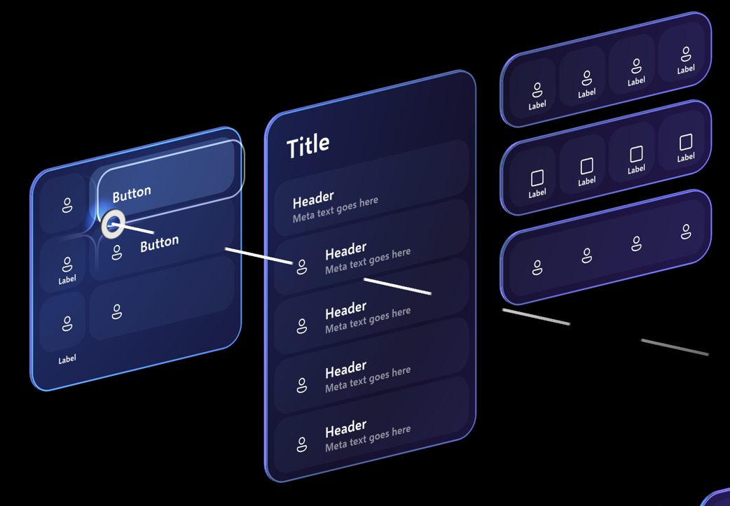
(Nearly) every button you generally work with in MRTK3 will be the same prefab. All UI elements are resizable and can be dynamically fit both to their surrounding containers and to the content they wrap. None of this is really an MRTK-specific invention; we’re just ensuring that all of our UX is built to the same standards that Unity’s own UI is built, with compatibility for all of the existing layout groups, constraints, and alignement systems.

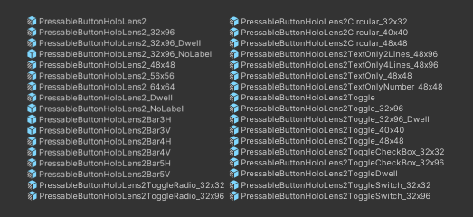
Every single button you see on this UI tearsheet is actually, in fact, the exact same prefab:

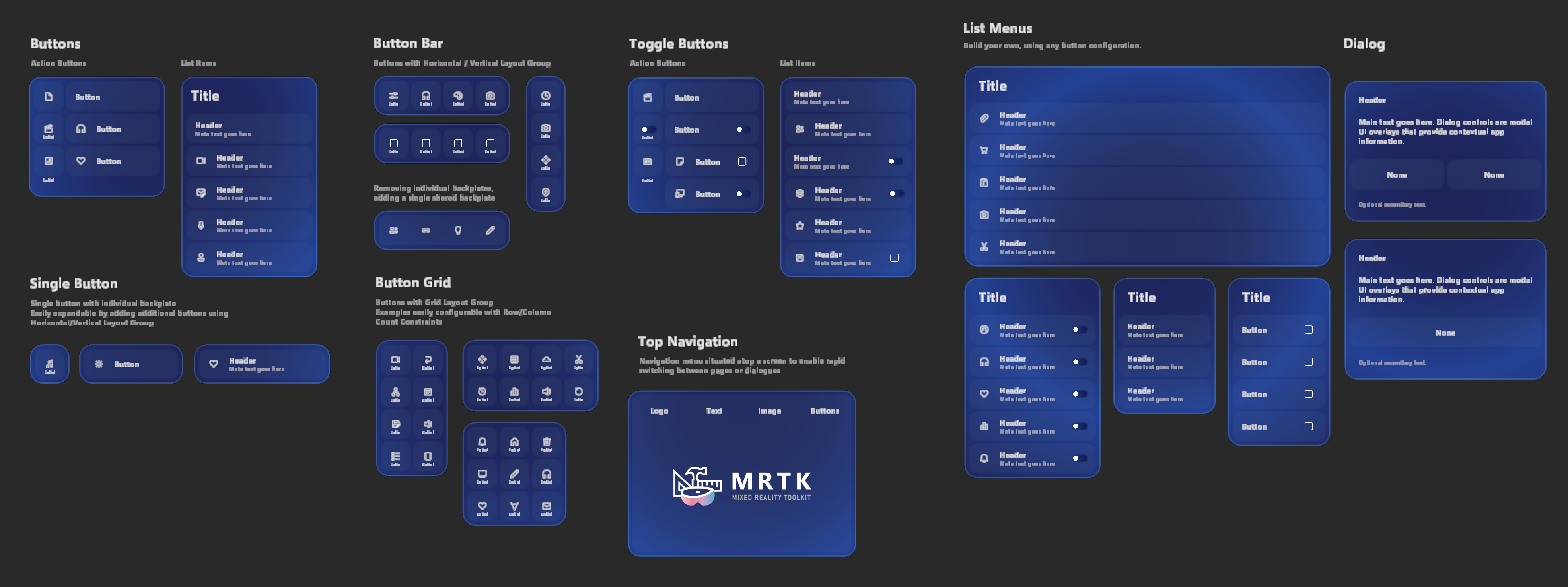
The speed at which designers can build UI templates is drastically accelerated. It’s actually fun, now, to build UI in MRTK… simple building blocks, combined together, to form more complex layouts.

Measurements

Another problem with working with UI at scale is that there are very specific requirements from the design language/library for measurements, both for usability concerns (minimum touch targets, readability, etc) as well as design (padding, margin, corner radii, branding). This was one of the most critical areas where our design in mixed reality had departed from the typical workflow that most designers are used to in 2D contexts. In the past, we had not only specified everything in absolute coordinates without any sort of flex or alignment parameters, but we used physical, real-world units for everything. All UI was designed in millimeters; branding guidelines were in millimeters, margin, padding, gutter, spacing, all in millimeters. Even fonts were specified in millimeters!

This had some advantages: notably, we were working in a real, physical environment. UI in mixed reality isn’t just some abstract piece of information on a screen somewhere; it’s essentially a real, physical object that exists in the real, physical world! It must have a defined physical size with physical units, at some point in the development process. We also have very strict requirements for usability with holograms; we have user research telling us that certain touch target sizes (32mm x 32mm, or 24mm at the absolute smallest) is acceptable for performing 3D volumetric pressing interactions with our fingers.

However, this attachment to physical units also had drawbacks. Primarily, this is an alien working environment to typical front-end designers, who are used to non-physical design units like em, rem, %, vh, or “physical” units that aren’t even really physical to begin with (px, pt). Traditional 2D design has a concept of DPI, or screen density, as well; but in mixed reality, there’s a much closer relationship between design and the physical world. (I like to think about it as something closer to industrial design, or physical product design: you’re building real, physical affordances that sit on a real, physical object!)

The most direct drawback was that in this system of everything being specified in absolute physical units, there was zero room at all for scaling. In mixed reality, there are still some circustances where the entire UI layout or design should be scaled up or down; this is common when reusing UI layouts for faraway, large objects (or reusing UI layouts for near or far interaction!) For UI elements like stroke, outline, and corner radius, we use shader-driven rendering techniques. When these are specified only in absolute physical units (like, say, a “1mm” stroke, or a “5mm” corner radius), there is no way for these measurements to remain proportionally consistent with the rest of your design. If your 32mm x 32mm button is scaled up 5x, your 1mm and 5mm design elements will still remain 1mm thick and 5mm wide. They will be proportionally incorrect, despite being specified in absolute units.

This gets pretty confusing, but the core of the issue is this: without RectTransforms or Canvas, there is no such thing as a dimension. There is only scale. For elements like stroke, or corner radius, we had to specify them “absolutely” so that they were consistent across the scaling operations used to adjust their size and shape. However, when the overall UI layout needed to be scaled up or down, those absolute measurements would become proportionally incorrect.

Here, let’s take a look at some visual examples to make this a bit less confusing. First, let’s see what happens to a non-RectTransform-based Dialog control when we want to “scale it up”:

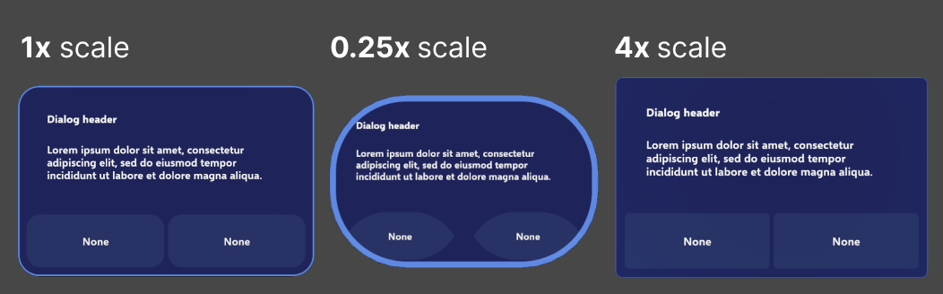
You can see that all of the strokes, corner radii, etc, that were absolutely specified in their physical units stayed “physically correct”; i.e., the strokes were always exactly 1mm. However, as the rest of the design scaled up and down, they became out of proportion!

You might say “just specify all of the elements as relative to the overall design scale… “ The issue is that, without RectTransform/Canvas, there is nothing to be relative to! If everything is just scaling operations on top of scaling operations, there’s no way to define any sort of true relative measurement. Every relative measurement would be relative to its parent, which would have any number of destructive scaling operations applied to it. There is no “root” of the design, and no “DPI” that could be used to specify a relative measurement unit.

How do you solve this? The answer is non-physical design units, with a certain “scale factor” (similar to a display’s DPI, except now we’re applying this to the relative size of a hologram to the physical world!). Non-physical units and design scale factors are only possible with Canvas and RectTransform layout, where the Canvas itself serves as a “design root”, and individual UI elements are not scaled, but instead sized.

UI is designed in an arbitrary, non-physical unit. Let’s call it u for now, for lack of a better name! (Internally, we generally call it px, but that’s quite the overloaded term… it’s not pixels, not on any actual physical device!)

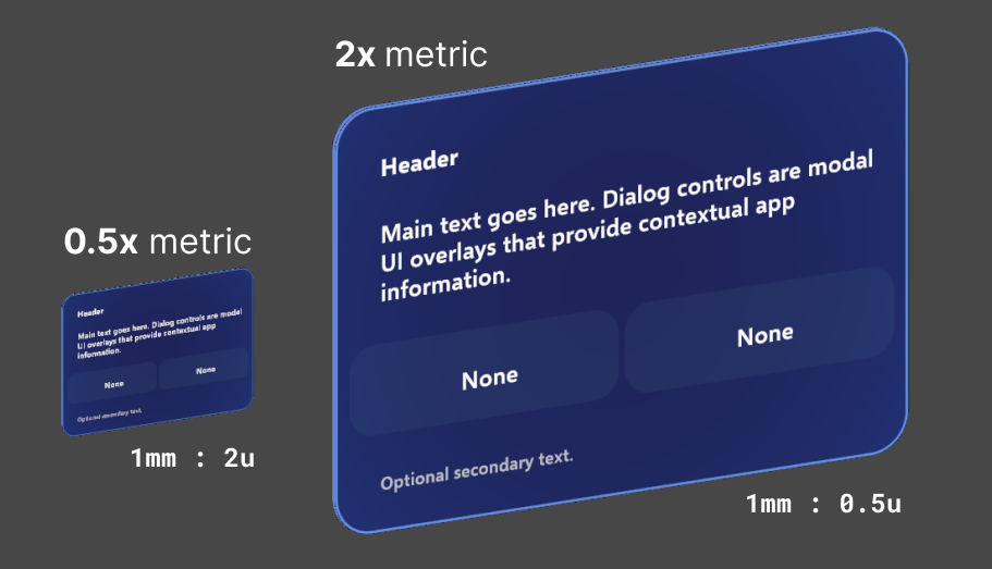
We’ll also define a scale factor, or metric. MRTK3’s component library uses a 1mm to 1u scale metric by default, but other component libraries at Microsoft have used other metrics, like 1mm to 3u. In MRTK3, our trusty 32mm button is now measured 32u x 32u. At the default scale (of 1mm : 1u) we get our standard, recommended 32mm touch target! However, most critically, we also have the freedom to rescale our measurements whenever we want, so we can scale up and down entire designs while maintaining design integrity.

Here’s a RectTransform-based Dialog control, showing how even when we scale it from 0.5x to 2x, all of the branding and visual elements remain proportionally correct.

Now, when designers build layouts in external tools like Figma, they can deliver redlines to engineers or tech designers that can actually be implemented! By using design units rather than physical units, along with powerful realtime layout, flex, and alignment systems, we can implement much more modern and robust designs without resorting to manual placement and napkin math.

Volumetric UI in a Flat World

Interacting with 3D user interfaces, while at the same time following traditional 2D interface “metaphors” like clipping and scrolling is difficult. Our UI controls in MRTK3 are fundamentally real, solid objects, with depth, volume, and thickness.

Containing these objects within UI metaphors like “scroll views” can be tricky; what does “clipping” look like in a volumetric context? Normally, UI has raycast/hit targets that are represented as 2D rectangles (or even alpha-tested bitmaps/hitmaps) that can overlay and intersect, and can be clipped by a 2D clipping rectangle.

With 3D, volumetric UI, what does that even look like? Unity UI generally functions with image-based raycast hit testing, as described above; that generally doesn’t cut it for our volumetric UI, as we need full, physicalized colliders for our 3D pressing interactions and free-form 3D layout. Colliders can’t easily be “clipped” like an image-based raycast target, right?

As part of our effort to adopt existing Unity UI constructs like LayoutGroups and RectTransform hierarchy-based clipping, we’ve developed systems to clip volumetric UI and its corresponding physical colliders in a component-for-component compatible way with the existing Unity UI scroll view system. Colliders are clipped in a depth-correct (planar) way that allows 3D UI with thickness and volume to accurately conform to the bounds of a Unity UI scrollview/clipping rectangle, even when objects and colliders are partially clipped, or intersecting the edges of the clipping region.

In previous iterations of MRTK, we’ve simply enabled or disabled colliders as they leave the footprint of the clipping region. This resulted in users accidentally pressing buttons that were 90% invisible/clipped, and buttons that were still visible being unresponsive. By accurately clipping colliders precisely to the bounds of the clipping region, we can have millimeter-accurate 3D UI interactions at the edge of a scroll view.

And, this is all based on the existing Unity UI layout groups and scroll components, so all of your scrolling physics remains intact, and is simultaneously compatible with traditional 2D input like mouse scroll wheels, multitouch trackpads, and touchscreens.

Input

Our 3D volumetric UI sits at the intersection of a huge number of input methods and platforms. Just in XR, you have

• Gaze-pinch interaction (eye gaze targeted, hand tracking pinch and commit), with variable/analog pinching input
• Hand rays, with variable/analog pinching input
• Pressing/poking with hand tracking (any number of fingers!), with volumetric displacement
• Gaze-speech (“See-It-Say-It”)
• Global speech (keyword-based)
• Motion controller rays (laser pointer), with analog input
• Motion controller poke (same volumetric displacement as hands!)
• Gaze dwell
• Spatial mouse (a la HoloLens 2 shell, Windows Mixed Reality shell)

The list expands even further when you consider flat-screen/2D input…

• Touchscreen/multitouch
• 2D mouse
• Gamepad
• Accessibility controllers
• Keyboard navigation

Unity’s UI systems are great at 2D input. They offer out-of-the-box touchscreen, mouse, and gamepad input. They even offer rudimentary point-and-click-based XR input. However, when you look at the diversity and richness of the XR input space we try to solve with MRTK, basic Unity UI input is unfortunately inadequate.

Unity UI input is fundamentally two-dimensional. The most obvious gap is with volumetric 3D pressing/poking interactions; sure, pointer events could be emulated from the intersection of a finger with a Canvas plane, but XR input is so much richer than that! Your finger can be halfway through a button, or your gaze-pinch interaction could be halfway-pinched, or maybe any number of combinations of hands, controllers, gaze, speech… When UI is a real, physical object with physical characteristics, dimensions, and volume, you need a richer set of interaction systems.

Thankfully, MRTK3 leverages the excellent XR Interaction Toolkit from Unity, which is an incredibly flexible framework for describing 3D interaction and manipulation. It’s more than powerful enough to describe all of our complex XR interactions, like poking, pressing, pinching, and gazing… but, it’s not nearly as equipped to handle traditional input like mice, touchscreens, or gamepads. Hypothetically, we could re-implement a large chunk of the gamepad or mouse input that Unity UI already provides, but that sounds pretty wasteful! What if we could combine the best parts of XRI’s flexibility with the out-of-the-box power of Unity’s UI input?

We do just that with our component library, in a delicate dance of adapters and conversions. Each MRTK3 UI control is both a UnityUI Selectable and an XRI Interactable, simultaneously! This gives us some serious advantages vs only being one or the other.

Our XRI-based interactors can perform rich, detailed, 3D interactions on our UI controls, including special otherwise-impossible behaviors like analog “selectedness” or “pressedness” (driven by pinching, analog triggers, or your finger pressing the surface of the button!). At the same time, however, we get touchscreen input, mouse input, and even directional gamepad navigation and input as well, without needing to implement any of the input handling ourselves.

We achieve this by translating incoming UnityUI events (from the Selectable) into instructions for XRI. The XRI Interactable is the final source of truth in our UI; the only “click” event developers need to subscribe to is the Interactable event. However, using a proxy interactor, we translate UnityUI events (like OnPointerDown) into an equivalent operation on the proxy interactor (like an XRI Select or Hover). That way, any UnityUI input, such as a touchscreen press or gamepad button press, is translated into an equivalent XRI event, and all codepaths converge to the same OnClicked or OnHoverEnter result.

The flow of how these events get propagated through the different input systems and interactors is detailed in this huge diagram… feel free to open in a new tab to read closer!

What this means for your UI is that you can use the exact same UI prefabs, the exact same events, and the exact same UI layouts across a staggeringly huge number of devices and platforms, all while retaining the rich, volumetric, delightful details that MRTK UX is known for.

Wrap-up

This post could go on for several dozen more pages about all of the new MRTK3 UX tooling and features… but, the best way to explore it is to go build! Check out our documentation for the new systems here, and learn how to set up your own new MRTK3 project here! Alternatively, you can directly check out our sample project by cloning this git repository at the mrtk3 branch here.

In the future, I’ll be writing some more guides, teardowns, and tutorials on building volumetric UI with the new tooling. In the meantime, you can check out my talk at MR Dev Days 2022, where I go over most of the topics in this post, plus a breakdown of building a real UI layout.

I hope you’ve enjoyed this deep dive into some of the new UI systems we’ve built for MRTK3, and we can’t wait to see what you build with our new tools. Personally, I love gorgeous, rich, expressive, and delightful UI, and I can’t wait to see all of the beautiful things that the community can cook up.

This summer, I’ve had the pleasure of working at Microsoft and contributing to MRTK. If you’re out of the loop, MRTK is one of the leading frameworks for building intuitive applications for AR and VR platforms, both Microsoft-owned (HoloLens, WMR, etc) and third-party platforms (Oculus, OpenVR/SteamVR, etc). It’s an open source effort, and it’s not one of those “open source” projects; we take significant PRs from real, unaffiliated third-party contributors, and our open philosophy is designed to help the entire AR industry effort as a whole. That being said, the following words are my own, and do not necessarily indicate the opinions of Microsoft or the MRTK team.

Elastic systems for interaction feedback

Harmonic oscillators are pretty awesome. They’re found everywhere in nature, they’re used in many existing interfaces, and they’re also just pretty damn fun. You’re probably most familiar with them in the form of a simple 1-dimensional spring, but damped oscillators can be so much more than that. Damped harmonic oscillators (we’ll call them elastic systems) can be extended to an arbitrary number of dimensions, applied to a huge range of outputs, and can be composed (i.e. one oscillator can drive another.) They’re also “haptically familiar” to most users; meaning that when a user picks up or plays with an object driven by a damped oscillator, it feels natural, familiar, and intuitive.

After all, the real world is not exact. Objects do not cling to your hand with perfect precision, your hands are not infinitely strong, and stretchy objects can slip away from your hands, too. Why do our virtual interfaces have to be always perfectly obedient?

Our users spend hours pulling, pushing, and poking virtual objects. Why can’t they push back?

Elastic feedback gives virtual objects their own “pull”; they can stretch, fling, squeeze, flip, wobble, and bounce. If the object is constrained by an elastic snap, it will linger and fight your input, stretching towards its goal, eventually flinging itself away and into your hand.

I’ll start with a visual tour, so that you have a bit of motivation to learn about the math behind these systems later! Firstly, one of the most fun things that can be done with the elastics are origami-style folding menus. By linking the output of the elastic sim with the rotations of these composable menu panels, some really exciting inflation/deflation effects can be achieved.

This could hypothetically be achieved with a hand-authored animation, but the elastic benefits this by being totally procedural (no artist-authoring needed), and reactive (if the button was pressed in the middle of the inflation, the panel would seamlessly deflate without needing to transition between animations).

Here, the flipping UI panel effect is combined with a scaling effect, constrained to hand/palm rotation and finger angle.

One of the greatest advantages of the elastic simulation system is the reactive, dynamic nature of the elastic systems. User input drives the elastic system, and the system will simulate the response of the elastic material to the user. Here, a drawstring-like element is driven by the user input to stretch, snap, and wobble into place.

The one-dimensional world is boring. We’re here to go boldly forth into the world of 3D interfaces, and 3D springs are here to help. From left to right, we have 3D snapping interval springs, a volume spring extent, and (gasp) a 4-dimensional quaternion spring (more on that later!)

The three-dimensional and four-dimensional elastic systems can be combined to drive fully elastic-enabled object manipulation.

Now that (I hope) you’re motivated by these fun examples, I’ll talk a little more about how they’re made and the math that drives them.

Damped harmonic oscillators are driven by a set of differential equations, which are configured by several values that describe the properties of the oscillator. Some of these values are inherent to the elastic “material” itself, but some of these values specify the extent or volume in which the elastic system lives. The values that configure the elastic material include the mass, drag, and spring constants associated with the system. There are three spring constants associated with each system; one is used for the forcing value, e.g., user input, another is used for the snapping force, and yet another is used to configure the strength of the end-limits of the extent. The relative magnitudes of these three constants dictate the snappiness, rigidity, and “feel” of the elastic-driven component.

// The inherent properties of the elastic behavior itself.
var elasticProperties = new ElasticProperties
{
    Mass = 0.03f,  // Mass of the elastic system
    HandK = 4.0f,  // Spring constant for the forcing factor
    EndK = 3.0f,   // Spring constant for the endcaps
    SnapK = 1.0f,  // Spring constant for the snap points
    Drag = 0.2f    // Damping
};

On the other hand, the values that configure the extent include the minimum/maximum extent, snapping points (“divots” in the extent that the spring will naturally tend to fall into) and snapping intervals (repeated snapping points that are tiled infinitely outwards in the extent.)

// A linear extent from 0.0f to 1.0f
var elasticExtent = new LinearElasticExtent
{
    MinStretch = 0.0f, // "Bottom" of the extent
    MaxStretch = 1.0f, // "Top" of the extent
    SnapPoints = new float[] { 0.25f, 0.5f, 0.75f },
    SnapRadius = 0.1f, // Maximum range of the snap force
    SnapToEnds = true  // Whether the ends are counted as snaps
};

If the system is stretched past the min or max end-cap, it will be forced back within the extent according to the EndK constant. If any snap points are configured, the system will experience a force driving it towards the nearest snap point, according to a polynomial function. You can play with the snap function here in the embedded Desmos graph; r is the radius of the snapping point, and k is the snapping spring constant.

Here, I’ve plotted the potential energy of the system against the snapping force; you can clearly see that if the elastic system were left to come to rest, it would slide into the snapping point’s energy well.

As we extend our elastic systems to higher dimensions, our extent also needs more information. For example, a volumetric 3D spring requires a 3D extent.

// A 3D extent centered at (0,0,0)
var elasticExtent = new VolumeElasticExtent
{
    StretchBounds = new Bounds
    (
        Vector3.zero, // Extent centered at (0,0,0)
        Vector3.one   // Cube-shaped, 1-unit wide
    ),
    UseBounds = true,
    SnapPoints = new Vector3[]
    {
        new Vector3(0.2f, 0.2f, 0.2f) // Snap interval
    },
    RepeatSnapPoints = true, // Snap point tiled across extent
    SnapRadius = 0.1f, // Maximum range of the snap force
};

Here, our 3D elastic system lives within a 3D extent. The extent centers around (0,0,0), and is one unit wide; UseBounds is true, so the bounds will be actively constraining the system. A single snap point at (0.2, 0.2, 0.2) is configured, but RepeatSnapPoints is true; this turns our single snapping point into a snap interval: the snapping point is “tiled” across the extent, resulting in an infinite number of snapping points all placed at integer multiples of the given snap point. So, this snap point generates snapping points spaced at 0.2-unit intervals. (This was how that 3D grid snapping system was implemented!)

Going even further down the rabbit hole (!), a quaternion elastic system requires a 4-dimensional extent. A quaternion spring operates along similar principles to the lower-dimensional systems, but displacements and forces are calculated as quaternions in 4-space, instead of vectors in 3-space.

// A 4D quaternion extent!
var elasticExtent = new QuaternionElasticExtent
{
    SnapPoints = new Vector3[]
    {
        new Vector3(45, 45, 45) // Euler angles
    },
    RepeatSnapPoints = true, // Snap point tiled across extent
    SnapRadius = 22.5f, // Maximum range of the snap force
};

Here, our quaternion extent appears quite similar to the volume extent; but instead of the snap points specified as 3D points in a bounding volume, they are specified as the Euler angles of the snap points along a sphere. The math is quite a bit more complicated internally, but give similarly intuitive results to the 1D and 3D implementations.

Driving these elastic systems is very easy; as they do not depend on Unity’s internal physics systems, you can call their ComputeIteration() method at any time, with any specified deltaTime. This allows you to compute many iterations in one frame (useful for unit testing your elastics!) as well as computing the equilibrium value of a system.

// Computes one Unity frame's worth of simulation time.
var newValue = myElastic.ComputeIteration(goalValue, Time.deltaTime);

// We can also compute the equilibrium, while using a custom timestep.
var simulationTimeStep = 0.1f; // Much bigger than Time.deltaTime!
while(myElastic.CurrentVelocity() > 0.001f)
{
    myElastic.ComputeIteration(goalValue, simulationTimeStep);
}

// Ta-da!
var equilibrium = myElastic.CurrentValue();

In some cases, you might like to let the elastic system come to rest, without any goal value. This is useful for when, say, the user lets go of an elastic-driven object. To do so, simply compute the iterations with the current value of the system as the goal value.

elasticValue = myElastic.ComputeIteration(elasticValue, Time.deltaTime);

You can check out the pull request that introduced most of these features here: GitHub

There’s been a pretty strong response from the developer community expressing their interest in including these elastic systems in their projects; I hope to hear more about the awesome stuff that people have built with elastic feedback. If you have something to share, feel free to email me or connect with me on LinkedIn or GitHub. Here’s to a better, springier future for mixed reality!

Last semester, I was fortunate enough to co-author a paper with my colleagues at the University of Illinois on benchmarking extended reality algorithms as part of our efforts towards a fully open-source XR ecosystem. In this paper, we profiled and benchmarked several standard XR components (SLAM/VIO for tracking, rotational reprojection, holographic reconstruction for multi-focal displays, among others) and made observations about the improvements that would be necessary for ideal AR/VR.

View our research paper on arXiv

Visit the ILLIXR project website

My portion of the work was dedicated to the post-processing/rotation reprojection. For AR/VR, reprojection is essential for improving motion-to-photon latency, as well as making up for poorly-performing applications and limited hardware resources. For our implementation, we ported several shaders from J.M.P. van Waveren’s famous source code from the original Oculus rotational timewarp implementation. We extracted the reprojection code to use in our own isolated benchmarking application. In addition, we also used the lens distortion correction and chromatic aberration correct shaders from van Waveren’s project as well; resulting in a full post-processing stack for typical VR HMDs.

Moving forward, we are working to create an entire, brand-new, open source, modular XR runtime for both academic researchers and XR hackers everywhere. We are building a rock solid foundation for high performance and modular XR solutions, using the Monado OpenXR interface for compatibility with up-and-coming OpenXR applications and game engines.

The LicheePi Zero is a lovely, tiny, single-board computer, running on the ubiquitous and low-cost Allwinner V3S platform. Extremely cheap single-board computers have exploded in popularity in recent years, even beyond the (in)famous Raspberry Pi. Other, smaller manufacturers have popped up, designing simple SBCs around inexpensive ARM SoCs. For hobbyists and hackers that want a more hands-on and challenging experience than you’d find with a Raspberry Pi, these cheap SoCs are a great hobby project and weekend adventure.

To add to the already significant challenge, most of the (sparse) documentation is in Chinese, and many of the necessary files are hosted on Chinese sites that are difficult to use or access from the States. While some challenges are technical in nature and can provide some value to the intrepid hobbyist, inaccessible documentation and unresponsive file-sharing sites are not the kind of issues I’d like to let stand. Thus, I wanted to share a guide for my English-speaking friends, serving as a concise tutorial for compiling the Linux kernel, a bootloader, and creating a root filesystem for the board.

Background

One of the main sources of reference for working with Allwinner SoC-based platforms will be linux-sunxi, an open source community that develops software for these low-cost single board computers. They have a great guide for compiling the various components for these boards, and also host a wide variety of repositories containing code specialized for these platforms. We’ll be using their configuration for u-boot, and some of the shell snippets I’ll share are borrowed from their guides.

The bootloader we’ll be using is the popular Das U-Boot, a basic bootloader designed to run on pretty much anything. Because the V3S SoC is well supported, we’ll be able to use the mainline, upstream U-Boot repository, with no need for any specialized Lichee or Sunxi forks.

For the kernel, we’ll be using the LicheePi fork of the Linux kernel. Theoretically, upstream Linux would work just fine, but I can’t find a configuration file for the V3S in the upstream repository. Lichee hosts a fork that includes a configuration file that I’ve found to work well, so we’ll use that. If you figure out the configuration file for the most recent upstream kernel, please let me know, and I can update this! Ideally, we ought to use the upstream versions of both U-Boot and the kernel, but we’ll settle for just using upstream U-Boot for now, and using Lichee’s Linux fork.

You should be using a relatively up-to-date version of Linux on your workstation; it’s possible to do some of this on Windows, but certain tasks like compiling U-Boot and the kernel are much more difficult on Windows. Personally, I try and use WSL for most tasks on my Windows workstation, but even WSL won’t be up to the task today. Either run a VM or create a Linux partition. You won’t need much disk space for this, the minimum disk space allocation should be fine.

Hardware

The LicheePi Zero is Lichee’s midrange SBC, powered by the Allwinner V3S SoC. The V3S was originally intended for dashcams, but has found a second life as a cheap SoC for hobbyist SBCs! The unit I have here was rougly $12 USD on Aliexpress, with international shipping included. To run Linux at 1.2 GHz, with integrated DDR2, a 3D graphics accelerator, floating point support, 40-pin LCD output, and more, all in the size of a thumb drive, for only $12? Sounds like a deal to me!

The V3S specs are below, as taken from the sunxi wiki:

• CPU: Cortex-A7 1.2GHz (ARM v7-A) Processor which have both VFPv3 and NEON co-processors:
• FPU: Vector Floating Point Unit (standard ARM VFPv4 FPU Floating Point Unit)
• SIMD: NEON (ARM’s extended general-purpose SIMD vector processing extension engine)
• Integrated 64MB DRAM

As a dashcam SoC, it has robust support for H.264 codecs at 1080p, which is quite remarkable for a sub-$5 chip.

You’ll need a few other bits of hardware, too: most importantly, you’ll need some way to talk to the UART on the board. The best way is to use an FTDI breakout board, variants of which are sold literally everywhere and can be found for just a few dollars. We’ll use this as our /dev/ttyUSB0 to talk to our board, both while we are working with the bootloader and when we’re talking to our Linux shell.

Additionally, we’ll be using an MicroSD card (sometimes referred to as a TF card, by some documentation) to flash the bootloader, kernel, and rootfs. The system can support a flash chip, but that’s outside the scope of this tutorial, for now. Some people say that larger-capacity MicroSD cards can cause issues; I’m using an old 8GB Kingston card for this tutorial, which hasn’t given me any issues. If you’re using one with capacity greater than, say, 32GB, and you’re having issues; maybe try a smaller one.

Toolchain

We need to install the compiler toolchain; one pitfall I ran into was that the V3S has hardware floating point support, unlike some other Allwinner chips (F1C100S, for instance). Therefore, we have to be careful to use the gcc-arm-linux-gnueabihf toolchain instead of the gcc-arm-linux-gnueabi toolchain. Install the toolchain like so:

$ sudo apt install gcc-arm-linux-gnueabihf

Make sure that your system is new enough that it downloads at least version >=6.0. U-Boot will not compile without a sufficiently new toolchain. I had to upgrade my ElementaryOS/Ubuntu installation to 18.04 for the included PPAs to have >=6.0.

U-Boot

First step is to compile our bootloader. We’ll be using the mainline, upstream U-Boot distribution, as the V3S is well-supported and requires no extra patches or special support. Clone the U-Boot repository with

$ git clone https://github.com/u-boot/u-boot.git
$ cd u-boot

You may need the swing and python-dev libraries. Install them before proceeding with the U-Boot compilation process.

$ sudo apt install swig python-dev

In order to compile U-Boot for our particular setup, we’ll use the configs/LicheePi_Zero_defconfig that Lichee provides as part of the mainline U-Boot repository we just cloned.

$ make CROSS_COMPILE=arm-linux-gnueabihf- LicheePi_Zero_defconfig

If that works, compile the bootloader:

$ make CROSS_COMPILE=arm-linux-gnueabihf-

If the system complains about not being able to find your toolchain, ensure you included the trailing hypen, as it will use the CROSS_COMPILE environment variable as a prefix to find the rest of the toolchain utilities (gcc, as, ld, etc).

If all goes well, the system should generate a file called u-boot-sunxi-with-spl.bin. This the bootloader binary, and we’ll copy this onto our SD card once we have the rest of the components ready.

Kernel

Next, we’ll compile the kernel. For this, we’ll need the Lichee fork of the Linux repository; they’ve kindly created a kernel configuration that works well on the board. It would be a long and arduous process to figure out the correct configuration on our own, so we’ll use this configuration for our kernel installation. As the Linux repo is very large with a deep Git history, we’ll do a shallow clone of depth=1 and only clone the particular branch we need:

$ git clone --single-branch --branch="zero-5.2.y" --depth=1 https://github.com/Lichee-Pi/linux.git
$ cd linux

This is the mainline Linux kernel, as of version 5.2, with a few changes; as I mentioned above, they added the configuration file for the LicheePi Zero, as well as the device tree (.dts) file and a useful touchscreen device driver. (We won’t use that in this tutorial, but it’s nice to have anyway.)

Make the configuration by running the following command. This will parse the kernel configuration and generate a .config that the main Make process will use to compile our kernel.

$ make ARCH=arm CROSS_COMPILE=arm-linux-gnueabihf- licheepi_zero_defconfig

If this succeeds, you’re ready to compile your kernel. Make note of how many threads/cores you’d like to assign to the job, and use the -j option to split the workload across them. For example, my system has 8 threads, so I’ll use -j8.

$ make ARCH=arm CROSS_COMPILE=arm-linux-gnueabihf- -j8 all

This will also compile the device tree. In a nutshell, the device’s hardware setup is described in the arch/arm/boot/dts/sun8i-v3s-licheepi-zero.dts file. The compilation process (with make all) will compile the .dts into a compiled, “binary” .dtb file that the bootloader/system can read. We’ll be copying this .dtb file over to our boot SD card, along with the zImage.

We’ll also need to compile/install the kernel modules. In my experience, the device boots fine without performing this step, but kernel modules are important and do need to be copied into the rootfs. Build the modules, and make sure INSTALL_MOD_PATH is set to some empty directory that you can access later. We’ll pull the module tree from this directory later.

$ sudo make ARCH=arm CROSS_COMPILE=arm-linux-gnueabihf- -j8 modules
$ sudo make ARCH=arm CROSS_COMPILE=arm-linux-gnueabihf- -j8 modules_install INSTALL_MOD_PATH=/path/to/some/directory

Boot script

To automate U-Boot’s boot process, we’ll create a small file that serves as an auto-running script. It contains a few U-Boot commands that will run when U-Boot initializes. Create a file called boot.cmd, containing the following U-Boot commands:

setenv bootargs console=ttyS0,115200 root=/dev/mmcblk0p2 rootwait panic=10
load mmc 0:1 0x43000000 ${fdtfile}
load mmc 0:1 0x42000000 zImage
bootz 0x42000000 - 0x43000000

Because the Sunxi wiki doesn’t explain these whatsoever, I’ll do the honors and break down each command and what purpose it serves.

setenv bootargs console=ttyS0,115200 root=/dev/mmcblk0p2 rootwait panic=10

This line sets the boot arguments, essentially a few short arguments we pass to the booting kernel to initialize a few options. To ensure the boot process outputs to the correct UART, we set the boot argument console=ttyS0,115200. This will ensure the critical boot debugging information is passed to UART0 at 115200 baud. This is usually what it would default to anyway, but it’s nice to be sure. root=/dev/mmcblk0p2 sets the root of the filesystem to the second partition of the SD card. This will become more clear later, but the second partition is the ext4 partition onto which we will load the actual rootfs (OS filesystem). rootwait ensures the boot process will stall and wait for the root storage medium to respond. This is important if the storage is being a bit slow. panic=10 tells the boot process to reboot/retry booting after 10 seconds if the kernel panics during boot.

load mmc 0:1 0x43000000 ${fdtfile}
load mmc 0:1 0x42000000 zImage

These commands load the .dtb file and zImage into memory from the SD card. The 0:1 identifier indicates we’re loading from mmc0, and we’re loading from the first (boot) partition. The .dtb file will be loaded into 0x43000000, and the kernel image will be loaded into 0x42000000. These are relatively arbitrary locations; they’re recommended for most of the Allwinner SoCs, but some use different load addresses. (For instance, the trimmed-down F1C100s SoC needs a high memory address like 0x80000000 and 0x80c00000 to load correctly.)

Finally, the bootz command boots the kernel, with three arguments specified; first, the kernel location, secondly, an option argument for the initramfs that we’re not using, and thirdly, the location of the .dtb file.

Once you’ve created the boot.cmd file with these commands, we’ll format this file into a .scr binary script file that U-Boot can use. Run the command:

$ mkimage -C none -A arm -T script -d boot.cmd boot.scr

The boot.scr file is what we’ll actually copy onto the SD card; boot.cmd will not be used.

Rootfs

The “rootfs” is the filesystem that is actually used by the operating system; it contains pretty much everything the operating system needs to provide the user (or root, in this case) with all the creature comforts that one expects while using a Linux system. It will contain binaries of common applications, like text editors, system utilities, as well as system files and programs.

There are several ways to create a rootfs. I’ve only had success with two methods, but that’s mostly due to my inexperience, rather than an actual technical limitation. The best method I’ve found is to use the excellent Buildroot utility to create a BusyBox-based rootfs that contains trimmed down versions of common Linux utilities. This is best suited for extremely resource-constrained systems; it won’t give you more advanced functionality like a C compiler, package management, or other features. However, the build process is painless, self contained, and relatively idiot-proof, lending itself well to a beginner’s tutorial.

Download the latest stable release of Buildroot, extract, and install the application.

We’ll select a few options for our Buildroot configuration. Run the menu-based configurator.

$ make menuconfig

Select the following options. If something else catches your eye, and you don’t think it would interfere with your system, feel free to select that too.

One particular area of note are the options for the included Busybox utilties. Busybox provides a set of commonly used utilities, but some are provided optionally.

A few that I’d like to recommend:

Once you’ve configured the Buildroot system with your favorite BusyBox utilities, build the filesystem:

$ make

Yes, it’s really that simple. This will take a good while (especially on slower systems), so, make a cup of tea, relax, and come back later. A few interesting notes while you’re waiting:

• Buildroot will use its own, internal, freshly downloaded compiler toolchain (if selected).
• Buildroot will resolve most, if not all, of its own internal dependencies at compile time.
• This helps builds be more reliable, less prone to weird package inconsistencies, and just be generally more convenient and idiot-proof!

Once the lengthy build process is complete, you’ll have a rootfs.tar file in your output folder. This is what we’ll un-archive into our SD card.

SD Card

We need to prep the card for use as a boot medium. Most of this is directly from the wonderful Sunxi bootable SD card guide, but I’ve edited it down to the steps that we need to perform for our project.

First, we need to mount and clean the SD card. Safe to say, anything on the card previously will be wiped, so please don’t use a card that is precious to you! If you’re used to working with removable storage on Linux, this will be old news, but here’s the boilerplate commands anyway.

The commands are slightly different depending on whether you’re using a USB-based external card reader, or an internally mounted MMC reader. I’m using a USB card reader, so when I run sudo fdisk -l to view the connected storage devices, I see my SD card as /dev/sdb. If you’re using a USB reader too, you’ll see your card as /dev/sdX, where X is some letter, depending on your configuration and if other SD devices are connected.

Make sure you identify the correct device. If you accidentally choose the incorrect device, you can permanently destroy data on another device, and irreversibly lose your information.

Once you’ve identified your device, export the name as as shell variable for easy use later.

$ export card=/dev/sdX

If the card is connected as a raw MMC device, it will probably appear as /dev/mmcblk0. Thus, export the variable as such:

$ export card=/dev/mmcblk0

Wipe the card’s partition table with the following command:

$ sudo dd if=/dev/zero of=${card} bs=1M count=1

If you’re not familiar with dd, the bs option indicates we’ll be writing a block of size 1M, and count=1 indicates we’ll be writing a single 1M block. if is the input, which will be /dev/zero as we’re zeroing out the partition table, and of is the output, which is our SD card. (Basic stuff, but still important.)

Next, we write the bootloader binary onto the device. Locate the u-boot-sunxi-with-spl.bin file we created earlier.

$ sudo dd if=/path/to/your/binfile/u-boot-sunxi-with-spl.bin of=${card} bs=1024 seek=8

Again, we’re using dd similarly as before, but this time our input is our .bin file, and we’re seeking 8 1024-byte blocks into the card, because the bootloader needs to start at 8K into the memory region of the card.

Next, we need to create a few partitions; notably, we’ll make a small boot partition that will hold our kernel zImage, the device tree binary, and the boot script.

• zImage is the kernel image we compiled earlier. It’s a compressed form of the binary, which is decompressed at boot.
• The device tree binary is that compiled .dtb file we generated earlier. It’s placed alongside the kernel image in the boot partition.
• The boot script, as described above, will be run by U-Boot at startup.

The layout of these partitions and the files within:

To create these partitions, we’ll use blockdev, which is a utility for controlling block devices, and sfdisk, a partition table utility.

$ sudo blockdev --rereadpt ${card}
$ cat <<EOT | sudo sfdisk ${card}
1,16,c
,,L
EOT

For those unaware, the sfdisk command behaves a little weirdly; you’ll type in the partition formatting after you run the second command, but they’re not commands: sfdisk just expects the formatting data as part of its standard input.

Creating the filesystems themselves is slightly different depending on whether you’ve mounted the SD card through a USB reader or as an MMC block device, so, only execute the one command that is relevant to your system.

Either MMC:

$ mkfs.vfat ${card}p1
$ mkfs.ext4 ${card}p2

or USB:

$ mkfs.vfat ${card}1
$ mkfs.ext4 ${card}2

Now that we have the partitions created, and the filesystems created within, it’s time to copy our files onto these filesystems. First, we mount the SD card’s boot partition to our host system. Again, the device name is slightly different depending on whether you’re using a USB reader or not; only execute one of these commands.

Either MMC:

$ sudo mount ${card}p1 /mnt/

or USB:

$ sudo mount ${card}1 /mnt/

Then, we copy our files to the boot partition.

$ sudo cp /path/to/your/linux/repo/arch/arm/boot/zImage /mnt/
$ sudo cp /path/to/your/script/boot.scr /mnt/
$ sudo cp /path/to/your/linux/repo/arch/arm/boot/dts/sun8i-v3s-licheepi-zero.dtb /mnt/

Then, sync all changes and unmount the SD card.

sync
sudo umount /dev/

At this point, you can actually remove the SD card, place it in your device, and boot to the bootloader! It’ll fail to boot the OS, of course, as we haven’t copied the rootfs yet, but it would be a good smoketest. Skip to the “FTDI/UART” section if you’d like to test this.

Next, we can mount the main ext4 partition and copy the rootfs we created.

Either MMC:

$ sudo mount ${card}p2 /mnt/

or USB:

$ sudo mount ${card}2 /mnt/

The rootfs that we built with Buildroot should be in the /path/to/your/buildroot/output/images folder. Remove it from the .tar and copy it to the SD card with:

$ tar -C /mnt/ -xf images/rootfs.tar

Inspect the SD card and verify that the root filesystem has been correctly extracted. Running ls /mnt/ should return something that looks generally like this:

bin  etc  lib32    media  opt   root  sbin  tmp  var
dev  lib  linuxrc  mnt    proc  run   sys   usr

If not, remove everything in the SD card (sudo rm -rf /mnt/*) and try again.

Next, we’ll copy over the kernel modules we compiled earlier. Recall the directory you compiled them into, and run the following commands:

sudo mkdir -p /mnt/lib/modules
sudo rm -rf /mnt/lib/modules/
sudo cp -r <YOUR_MODULE_DIRECTORY>/output/lib /mnt/

The rm -rf will simply clean the existing /mnt/lib/modules folder if one exists. If you’ve been following the tutorial, the rootfs we built with Buildroot does not include any in the image; so this is unnecessary. However, if you were using some other rootfs from some other source, there may be some pre-existing files. Removing them will provide a clean slate for us.

The rootfs copying process is now done! If everything worked correctly, you should now have a fully functioning SD card for your device.

Sync and unmount the SD card when you’re done.

sync
sudo umount /dev/

FTDI/UART

The time has come; we can now boot our system and see the fruits of our effort. Plug in and install your FTDI breakout (or other serial adapter solution) on the workstation. We’ll be using minicom as a feature-rich and easy-to-use serial monitor; there are a plethora of other ways to talk to a serial port, but I’ve found minicom to be excellent. Install it with your package manager of choice if you don’t already have it.

Run minicom and configure the terminal to use /dev/ttyUSB0 (for an FTDI breakout) with 115200 baud, 8N1, with no hardware flow control or software flow control. You can access the minicom serial configuration menu by pressing ctrl-A, then Z, after running it. Open the configuration with O, navigate to “Serial port setup” and verify your serial settings look like the picture.

+------------------------------------------+
| A -    Serial Device      : /dev/ttyUSB0 |
| B - Lockfile Location     : /var/lock    |
| C -   Callin Program      :              |
| D -  Callout Program      :              |
| E -    Bps/Par/Bits       : 115200 8N1   |
| F - Hardware Flow Control : No           |
| G - Software Flow Control : No           |
|                                          |
|    Change which setting?                 |
+------------------------------------------+

Once the serial port has been configured, connect your serial adapter to the board. Look for the pins labeled U0T and R. These are the Tx and Rx pins, respectively, of the default UART0. Connect the serial adapter (Tx to Rx, and Rx to Tx), and plug the LicheePi Zero into USB power.

If everything is normal, you should first see the U-Boot terminal briefly, before it auto-boots into our system. You should see a string of kernel boot messages, before you’re dumped to a root terminal.

If you’d like to sanity check your boot logs against what I have, please see this Gist. This is what my LicheePi Zero spits out on boot, using the kernel, U-Boot, and rootfs described in this tutorial.

Time to explore

Have fun with your Busybox environment! You can set a fun message of the day (displayed on bootup) by creating a file in /etc/motd. The popular editor vi should be installed by default, but it is a stripped down version and does not include most of the creature comforts you’d expect from a full vi installation. Explore the filesystem, play some games, write some Micropython scripts, and practice your shell scripting skills. One fun exercise is to run a script or program and use top or htop (if you included it in the Busybox configuration) to inspect how much system resources are being used.

GPIO

GPIO support is included, which allows you to play with the RGB LED mounted on the board. I wrote a small shell script that illustrates how to enable the GPIO, and write various values. If your board is configured similarly to mine, this should cause the RGB LED to flash different colors for an entertaining light show. GPIOs 192, 193, and 194 are the three color channels of the LED.

#!/bin/sh

echo 192 > /sys/class/gpio/export
echo 193 > /sys/class/gpio/export
echo 194 > /sys/class/gpio/export

echo out > /sys/class/gpio/gpio192/direction
echo out > /sys/class/gpio/gpio193/direction
echo out > /sys/class/gpio/gpio194/direction

for i in $(seq 1 1000);
do
        echo 0 > /sys/class/gpio/gpio193/value
        sleep 0.08
        echo 1 > /sys/class/gpio/gpio193/value
        echo 0 > /sys/class/gpio/gpio194/value
        sleep 0.08
        echo 1 > /sys/class/gpio/gpio194/value
        echo 0 > /sys/class/gpio/gpio192/value
        sleep 0.08
        echo 1 > /sys/class/gpio/gpio192/value
done

For extra fun you can make this a startup script, so that you can impress your friends and family (not really, who am I kidding) with your script without needing to log in. (Run this on the LicheePi, of course.)

First, mark the script as executable (you probably already did this)

$ chmod +x /path/to/your/script/your_script

At the end of the file named rcS in /etc/init.d, append the line

./path/to/your/script/your_script &

Save the file and restart the device. Your script should now begin running, even before root logs in. If your script was my blinky script above, you should be able to see the wonderful blinky lightshow immediately.

Have you ever felt the need to emulate RISC-V binaries on the most resource-constrained of platforms? Me neither, up until a few months ago. To help with another project, I decided to write a tiny RISC-V interpreter. It was especially timely as I was also taking a hardware design course where we implemented a RISC-V32IM core, so the ISA was fresh in my mind.

Features

The interpreter emulates real RISC-V binaries; it takes a stripped sequence of real RV32I machine code and disassembles, parses, and executes it, illustrating register file state and memory accesses as it runs. The most notable feature is that the main interpreter core is entirely stateless; the wrapper program is charged with storing processor state, which it simply passes to the interpreter, along with a pointer to a struct in which it will store the next execution state.

Therefore, a peculiar and quite useful use case emerges; the wrapper program can hold a circular buffer of execution state, allowing for arbitrary “unwinding” of execution history. In fact, this was the main selling point of the interpreter for the project I built it for; the user could quite literally “rewind time” by spinning a knob, watching the execution history roll backwards in realtime.

The entire thing is written in bare metal, portable C. This results in very efficient performance, a tiny executable size, and the ability to run the interpreter on pretty much any platform known to man. Our team ended up running the interpreter bare-metal on an STM32 microcontroller.

Why?

Why? Excellent question, but sometimes we do things just to say we can. It’s also quite the sight to see an STM32 running RISC-V binaries.

Clone the repository now, and emulate RV32I on all your favorite tiny devices today.