This summer, I’ve had the pleasure of working at Microsoft and contributing to MRTK. If you’re out of the loop, MRTK is one of the leading frameworks for building intuitive applications for AR and VR platforms, both Microsoft-owned (HoloLens, WMR, etc) and third-party platforms (Oculus, OpenVR/SteamVR, etc). It’s an open source effort, and it’s not one of those “open source” projects; we take significant PRs from real, unaffiliated third-party contributors, and our open philosophy is designed to help the entire AR industry effort as a whole. That being said, the following words are my own, and do not necessarily indicate the opinions of Microsoft or the MRTK team.

Elastic systems for interaction feedback

Harmonic oscillators are pretty awesome. They’re found everywhere in nature, they’re used in many existing interfaces, and they’re also just pretty damn fun. You’re probably most familiar with them in the form of a simple 1-dimensional spring, but damped oscillators can be so much more than that. Damped harmonic oscillators (we’ll call them elastic systems) can be extended to an arbitrary number of dimensions, applied to a huge range of outputs, and can be composed (i.e. one oscillator can drive another.) They’re also “haptically familiar” to most users; meaning that when a user picks up or plays with an object driven by a damped oscillator, it feels natural, familiar, and intuitive.

After all, the real world is not exact. Objects do not cling to your hand with perfect precision, your hands are not infinitely strong, and stretchy objects can slip away from your hands, too. Why do our virtual interfaces have to be always perfectly obedient?

Our users spend hours pulling, pushing, and poking virtual objects. Why can’t they push back?

Elastic feedback gives virtual objects their own “pull”; they can stretch, fling, squeeze, flip, wobble, and bounce. If the object is constrained by an elastic snap, it will linger and fight your input, stretching towards its goal, eventually flinging itself away and into your hand.

I’ll start with a visual tour, so that you have a bit of motivation to learn about the math behind these systems later! Firstly, one of the most fun things that can be done with the elastics are origami-style folding menus. By linking the output of the elastic sim with the rotations of these composable menu panels, some really exciting inflation/deflation effects can be achieved.

This could hypothetically be achieved with a hand-authored animation, but the elastic benefits this by being totally procedural (no artist-authoring needed), and reactive (if the button was pressed in the middle of the inflation, the panel would seamlessly deflate without needing to transition between animations).

Here, the flipping UI panel effect is combined with a scaling effect, constrained to hand/palm rotation and finger angle.

One of the greatest advantages of the elastic simulation system is the reactive, dynamic nature of the elastic systems. User input drives the elastic system, and the system will simulate the response of the elastic material to the user. Here, a drawstring-like element is driven by the user input to stretch, snap, and wobble into place.

The one-dimensional world is boring. We’re here to go boldly forth into the world of 3D interfaces, and 3D springs are here to help. From left to right, we have 3D snapping interval springs, a volume spring extent, and (gasp) a 4-dimensional quaternion spring (more on that later!)

The three-dimensional and four-dimensional elastic systems can be combined to drive fully elastic-enabled object manipulation.

Now that (I hope) you’re motivated by these fun examples, I’ll talk a little more about how they’re made and the math that drives them.

Damped harmonic oscillators are driven by a set of differential equations, which are configured by several values that describe the properties of the oscillator. Some of these values are inherent to the elastic “material” itself, but some of these values specify the extent or volume in which the elastic system lives. The values that configure the elastic material include the mass, drag, and spring constants associated with the system. There are three spring constants associated with each system; one is used for the forcing value, e.g., user input, another is used for the snapping force, and yet another is used to configure the strength of the end-limits of the extent. The relative magnitudes of these three constants dictate the snappiness, rigidity, and “feel” of the elastic-driven component.

// The inherent properties of the elastic behavior itself.
var elasticProperties = new ElasticProperties
{
    Mass = 0.03f,  // Mass of the elastic system
    HandK = 4.0f,  // Spring constant for the forcing factor
    EndK = 3.0f,   // Spring constant for the endcaps
    SnapK = 1.0f,  // Spring constant for the snap points
    Drag = 0.2f    // Damping
};

On the other hand, the values that configure the extent include the minimum/maximum extent, snapping points (“divots” in the extent that the spring will naturally tend to fall into) and snapping intervals (repeated snapping points that are tiled infinitely outwards in the extent.)

// A linear extent from 0.0f to 1.0f
var elasticExtent = new LinearElasticExtent
{
    MinStretch = 0.0f, // "Bottom" of the extent
    MaxStretch = 1.0f, // "Top" of the extent
    SnapPoints = new float[] { 0.25f, 0.5f, 0.75f },
    SnapRadius = 0.1f, // Maximum range of the snap force
    SnapToEnds = true  // Whether the ends are counted as snaps
};

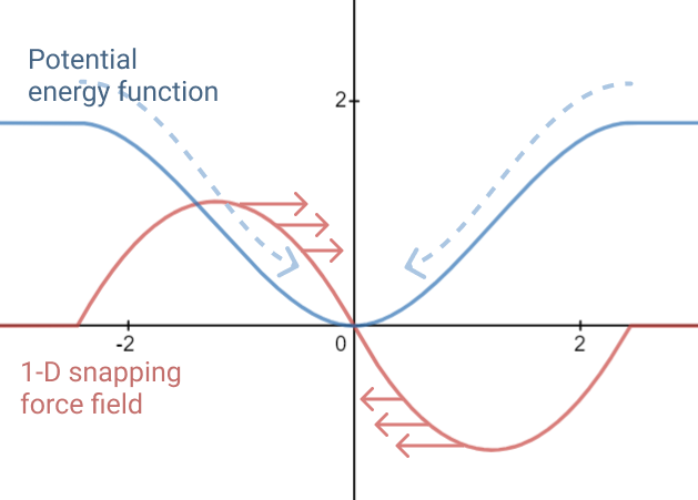
If the system is stretched past the min or max end-cap, it will be forced back within the extent according to the EndK constant. If any snap points are configured, the system will experience a force driving it towards the nearest snap point, according to a polynomial function. You can play with the snap function here in the embedded Desmos graph; r is the radius of the snapping point, and k is the snapping spring constant.

Here, I’ve plotted the potential energy of the system against the snapping force; you can clearly see that if the elastic system were left to come to rest, it would slide into the snapping point’s energy well.

As we extend our elastic systems to higher dimensions, our extent also needs more information. For example, a volumetric 3D spring requires a 3D extent.

// A 3D extent centered at (0,0,0)
var elasticExtent = new VolumeElasticExtent
{
    StretchBounds = new Bounds
    (
        Vector3.zero, // Extent centered at (0,0,0)
        Vector3.one   // Cube-shaped, 1-unit wide
    ),
    UseBounds = true,
    SnapPoints = new Vector3[]
    {
        new Vector3(0.2f, 0.2f, 0.2f) // Snap interval
    },
    RepeatSnapPoints = true, // Snap point tiled across extent
    SnapRadius = 0.1f, // Maximum range of the snap force
};

Here, our 3D elastic system lives within a 3D extent. The extent centers around (0,0,0), and is one unit wide; UseBounds is true, so the bounds will be actively constraining the system. A single snap point at (0.2, 0.2, 0.2) is configured, but RepeatSnapPoints is true; this turns our single snapping point into a snap interval: the snapping point is “tiled” across the extent, resulting in an infinite number of snapping points all placed at integer multiples of the given snap point. So, this snap point generates snapping points spaced at 0.2-unit intervals. (This was how that 3D grid snapping system was implemented!)

Going even further down the rabbit hole (!), a quaternion elastic system requires a 4-dimensional extent. A quaternion spring operates along similar principles to the lower-dimensional systems, but displacements and forces are calculated as quaternions in 4-space, instead of vectors in 3-space.

// A 4D quaternion extent!
var elasticExtent = new QuaternionElasticExtent
{
    SnapPoints = new Vector3[]
    {
        new Vector3(45, 45, 45) // Euler angles
    },
    RepeatSnapPoints = true, // Snap point tiled across extent
    SnapRadius = 22.5f, // Maximum range of the snap force
};

Here, our quaternion extent appears quite similar to the volume extent; but instead of the snap points specified as 3D points in a bounding volume, they are specified as the Euler angles of the snap points along a sphere. The math is quite a bit more complicated internally, but give similarly intuitive results to the 1D and 3D implementations.

Driving these elastic systems is very easy; as they do not depend on Unity’s internal physics systems, you can call their ComputeIteration() method at any time, with any specified deltaTime. This allows you to compute many iterations in one frame (useful for unit testing your elastics!) as well as computing the equilibrium value of a system.

// Computes one Unity frame's worth of simulation time.
var newValue = myElastic.ComputeIteration(goalValue, Time.deltaTime);

// We can also compute the equilibrium, while using a custom timestep.
var simulationTimeStep = 0.1f; // Much bigger than Time.deltaTime!
while(myElastic.CurrentVelocity() > 0.001f)
{
    myElastic.ComputeIteration(goalValue, simulationTimeStep);
}

// Ta-da!
var equilibrium = myElastic.CurrentValue();

In some cases, you might like to let the elastic system come to rest, without any goal value. This is useful for when, say, the user lets go of an elastic-driven object. To do so, simply compute the iterations with the current value of the system as the goal value.

elasticValue = myElastic.ComputeIteration(elasticValue, Time.deltaTime);

You can check out the pull request that introduced most of these features here: GitHub

There’s been a pretty strong response from the developer community expressing their interest in including these elastic systems in their projects; I hope to hear more about the awesome stuff that people have built with elastic feedback. If you have something to share, feel free to email me or connect with me on LinkedIn or GitHub. Here’s to a better, springier future for mixed reality!